This tutorial demonstrates how to merge data cubes using linked data frames.
For brevity the code used to construct the input cubes is hidden. You can read the details in the source code for this vignette on github.
There are a several ways to combine data cubes:
- concatenating rows to gather observations from different cubes into a single collection
- using correspondence lookups to translate dimension values from one codelist into another
- joining cubes by dimension and code URIs to add more rows or columns as required
We’ll explore each in turn.
Concatenating rows of observations
You can concatenate observations by “row binding” tables - adding rows from one table onto the end of another making a single, longer table.
This is simple if the cubes have the same components. This basically means that tables need to have the same set of columns.
Rows with matching columns
The following two excerpts from population datasets on linked.nisra.gov.uk have the same structure.
One is for Local Government Districts:
kable(pop_by_lgd)
| area | gender | age | population |
|---|---|---|---|
| N09000001 | All Persons | 0 | 1629 |
| N09000001 | All Persons | 1 | 1672 |
| N09000001 | All Persons | 2 | 1710 |
| N09000001 | All Persons | 3 | 1861 |
| N09000001 | All Persons | 4 | 1816 |
| N09000001 | All Persons | 5 | 1845 |
| N09000001 | All Persons | 6 | 1907 |
| N09000001 | All Persons | 7 | 2006 |
| N09000001 | All Persons | 8 | 1988 |
| N09000001 | All Persons | 9 | 2004 |
The other for Parliamentary Constituencies:
kable(pop_by_pc)
| area | gender | age | population |
|---|---|---|---|
| N06000001 | All Persons | 0 | 1141 |
| N06000001 | All Persons | 1 | 1163 |
| N06000001 | All Persons | 2 | 1170 |
| N06000001 | All Persons | 3 | 1159 |
| N06000001 | All Persons | 4 | 1150 |
| N06000001 | All Persons | 5 | 1205 |
| N06000001 | All Persons | 6 | 1135 |
| N06000001 | All Persons | 7 | 1186 |
| N06000001 | All Persons | 8 | 1233 |
| N06000001 | All Persons | 9 | 1153 |
These cubes are essentially the same, it’s just the there are different types of geography in the area column. Because the URIs for the two geography types can’t overlap (they’re Unique Resource Identifiers after all), we can concatenate the rows into a single table.
We need to use vctrs::vec_rbind() instead of base::rbind() because this makes sure the resource descriptions are merged:
| area | gender | age | population |
|---|---|---|---|
| N09000001 | All Persons | 0 | 1629 |
| N09000001 | All Persons | 1 | 1672 |
| N09000001 | All Persons | 2 | 1710 |
| N09000001 | All Persons | 3 | 1861 |
| N09000001 | All Persons | 4 | 1816 |
| N09000001 | All Persons | 5 | 1845 |
| N09000001 | All Persons | 6 | 1907 |
| N09000001 | All Persons | 7 | 2006 |
| N09000001 | All Persons | 8 | 1988 |
| N09000001 | All Persons | 9 | 2004 |
| N06000001 | All Persons | 0 | 1141 |
| N06000001 | All Persons | 1 | 1163 |
| N06000001 | All Persons | 2 | 1170 |
| N06000001 | All Persons | 3 | 1159 |
| N06000001 | All Persons | 4 | 1150 |
| N06000001 | All Persons | 5 | 1205 |
| N06000001 | All Persons | 6 | 1135 |
| N06000001 | All Persons | 7 | 1186 |
| N06000001 | All Persons | 8 | 1233 |
| N06000001 | All Persons | 9 | 1153 |
Rows with different columns
If the cubes have different structures we will need to alter the tables of observations so that they have the same columns. We can remove spare columns if we first filter the rows such that there’s only a single value for that column. We can add missing columns by filling in values with a default.
These two excerpts from the Journey times to key services datasets demonstrate the problem.
These are the journey times from each neighbourhood to the town centre:
kable(jt_town)
| area | mode | date | travel_time | unit |
|---|---|---|---|---|
| E01000001 | PT/walk | 2017 | 22.72201 | Minutes |
| E01000001 | Cycle | 2017 | 13.94595 | Minutes |
| E01000001 | Car | 2017 | 14.58818 | Minutes |
The employment centres table by contrast has one extra column: employment_centre_size. This breakdown wasn’t applicable to town centres but it’s important to distinguish employment centres.
kable(jt_employment)
| area | employment_centre_size | mode | date | travel_time | unit |
|---|---|---|---|---|---|
| E01000001 | Employment centre with 100 to 499 jobs | PT/walk | 2017 | 20 | Minutes |
| E01000001 | Employment centre with 100 to 499 jobs | Cycle | 2017 | 12 | Minutes |
| E01000001 | Employment centre with 100 to 499 jobs | Car | 2017 | 13 | Minutes |
| E01000001 | Employment centre with 500 to 4999 jobs | PT/walk | 2017 | 4 | Minutes |
| E01000001 | Employment centre with 500 to 4999 jobs | Cycle | 2017 | 7 | Minutes |
| E01000001 | Employment centre with 500 to 4999 jobs | Car | 2017 | 7 | Minutes |
We could choose to ignore it, picking a single value from the breakdown. In some cases the codelist will be hierarchical, having e.g. a value for “Any” or “Total” at the top of the tree. This effectively ignores the breakdown 1. In this case that’s not possible so we’ll have to pick an employment centre size.
Let’s take moderately-sized employment centres. Once we’ve filtered to those rows, we can remove the redundant column:
jt_employment_500 <-
   filter(jt_employment,
          label(employment_centre_size)=="Employment centre with 500 to 4999 jobs") %>%
   select(!employment_centre_size)

kable(jt_employment_500)
| area | mode | date | travel_time | unit |
|---|---|---|---|---|
| E01000001 | PT/walk | 2017 | 4 | Minutes |
| E01000001 | Cycle | 2017 | 7 | Minutes |
| E01000001 | Car | 2017 | 7 | Minutes |
We can then concatenate this with jt_town. If we do this now, however, there won’t be a way to distinguish between the rows that come from each dataset. The destination of the service being travelled to is defined only in metadata (i.e. by the dataset’s title) and isn’t available in the data to let the observations distinguish themselves 2. We need to add this column in ourselves:
jt_town <- mutate(jt_town,
                  destination="Town Centre")
jt_employment_500 <- mutate(jt_employment_500,
                            destination="Employment Centre (500-4999 jobs)")

vec_rbind(jt_town, jt_employment_500) %>% kable()
| area | mode | date | travel_time | unit | destination |
|---|---|---|---|---|---|
| E01000001 | PT/walk | 2017 | 22.72201 | Minutes | Town Centre |
| E01000001 | Cycle | 2017 | 13.94595 | Minutes | Town Centre |
| E01000001 | Car | 2017 | 14.58818 | Minutes | Town Centre |
| E01000001 | PT/walk | 2017 | 4.00000 | Minutes | Employment Centre (500-4999 jobs) |
| E01000001 | Cycle | 2017 | 7.00000 | Minutes | Employment Centre (500-4999 jobs) |
| E01000001 | Car | 2017 | 7.00000 | Minutes | Employment Centre (500-4999 jobs) |
Alternatively we can add the column to jt_town. Indeed vctrs::vec_rbind() will automatically set this to NA for us:
jt_employment <- mutate(jt_employment, destination="Employment Centre")

vec_rbind(jt_town, jt_employment) %>% kable()
| area | mode | date | travel_time | unit | destination | employment_centre_size |
|---|---|---|---|---|---|---|
| E01000001 | PT/walk | 2017 | 22.72201 | Minutes | Town Centre | NA |
| E01000001 | Cycle | 2017 | 13.94595 | Minutes | Town Centre | NA |
| E01000001 | Car | 2017 | 14.58818 | Minutes | Town Centre | NA |
| E01000001 | PT/walk | 2017 | 20.00000 | Minutes | Employment Centre | Employment centre with 100 to 499 jobs |
| E01000001 | Cycle | 2017 | 12.00000 | Minutes | Employment Centre | Employment centre with 100 to 499 jobs |
| E01000001 | Car | 2017 | 13.00000 | Minutes | Employment Centre | Employment centre with 100 to 499 jobs |
| E01000001 | PT/walk | 2017 | 4.00000 | Minutes | Employment Centre | Employment centre with 500 to 4999 jobs |
| E01000001 | Cycle | 2017 | 7.00000 | Minutes | Employment Centre | Employment centre with 500 to 4999 jobs |
| E01000001 | Car | 2017 | 7.00000 | Minutes | Employment Centre | Employment centre with 500 to 4999 jobs |
The following sections are a work in progress
Using correspondence lookups
The components ought to have compatible values too. We can mix codes from different codelists (skos:Concept URIs from different skos:ConceptSchemes) in the same column, but it is generally nicer to work with a common set.
This is particularly true if the scope of the codelists overlaps. If you can derive a single codelist with a set of mutually exclusive and comprehensively exhaustive codes, then it’s possible to aggregate the values without double-counting or gaps.
We can use correspondence tables to lookup equivalent values from one codelist in another.
# example with correspondence table
# Map SITC to CPA at highest level?
Join cubes by dimension and code URIs
If two cubes use the same codelist (or have dimensions with common patterns for URIs like intervals or geographies) then it’s possible to join them on that basis.
If every dimension is common to both cube codes (or if it only a single value), then it’s possible to do a full join using all the dimensions. This will result in a combined cube with the same set of dimensions (which uniquely identify the rows) and two values - one from each of the original cubes.
If these values are distinguished by dimension values, then they will be on different rows. Otherwise, the values could be put into different columns on the same rows. It’s possible to transform the data between these two representations using the tidyr package as described in the Tabulating DataCubes vignette. The longer (row bound) form is nicer for analysis (e.g. modelling or charting) whereas the wider (column bound) form is nicer for calculations that compare the values (e.g. denomination).
We’ll use two tables from Eurostat for this example. The first describes the total number of people employed in each country (in thousands):
| country | employment |
|---|---|
| Austria | 4148 |
| Belgium | 4708 |
| Bulgaria | 3121 |
The second describes the economically active population of each country (in thousands):
| country | population |
|---|---|
| Austria | 4336 |
| Belgium | 4969 |
| Bulgaria | 3258 |
Both have a country dimension that uses the same codes. We can use them together to calculate the employment rate.
If we combine them by column-binding we create a single, wider table 3.
emp_pop_wide <- dplyr::inner_join(employment, population, by="country")

kable(head(emp_pop_wide))
| country | employment | population |
|---|---|---|
| Austria | 4148 | 4336 |
| Belgium | 4708 | 4969 |
| Bulgaria | 3121 | 3258 |
| Switzerland | 4321 | 4515 |
| Cyprus | 400 | 431 |
| Czechia | 5126 | 5230 |
This form is convenient where we want to address the two variables with metadata.
For example, we can calculate the employment rate by referring to each variable:
emp_pop_wide %>%
   mutate(employment_rate = employment / population) %>%
   arrange(-employment_rate) %>%
   slice_head(n=5) %>%
   kable()
| country | employment | population | employment_rate |
|---|---|---|---|
| Czechia | 5126 | 5230 | 0.9801147 |
| Netherlands | 8077 | 8328 | 0.9698607 |
| Germany (until 1990 former territory of the FRG) | 39955 | 41234 | 0.9689819 |
| Malta | 245 | 253 | 0.9683794 |
| Iceland | 180 | 186 | 0.9677419 |
Alternatively, we can row-bind the tables to form a single, longer table. We have to add another dimension - variable - to the table to distinguish the rows from each source. This allows us to combine the employment and population measures into a single measure which simply counts people.
emp_pop_long <- rbind(
   transmute(employment, country, indicator="Employment", people=employment),
   transmute(population, country, indicator="Population", people=population)
   )

emp_pop_long %>%
   arrange(country) %>%
   slice_head(n=10) %>%
   kable()
| country | indicator | people |
|---|---|---|
| Austria | Employment | 4148 |
| Austria | Population | 4336 |
| Belgium | Employment | 4708 |
| Belgium | Population | 4969 |
| Bulgaria | Employment | 3121 |
| Bulgaria | Population | 3258 |
| Switzerland | Employment | 4321 |
| Switzerland | Population | 4515 |
| Cyprus | Employment | 400 |
| Cyprus | Population | 431 |
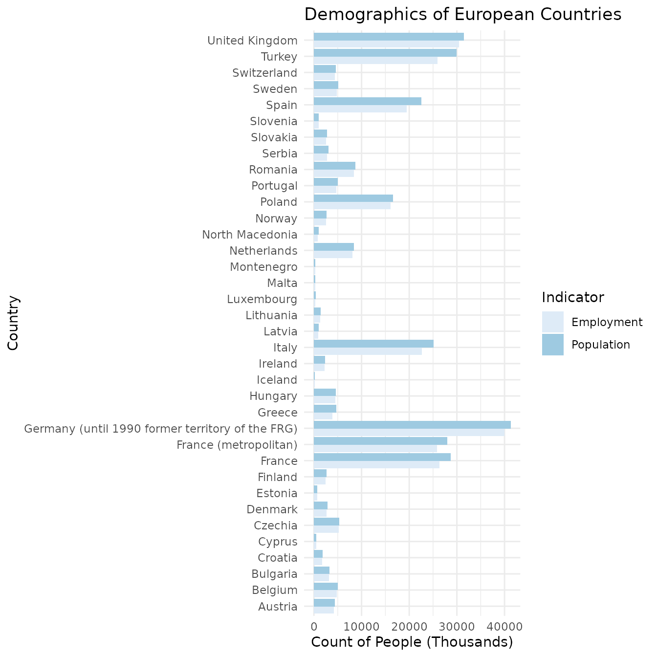
This form is convenient where we want to address the two variables as data.
For example, we can plot employment against population:
library(ggplot2)

ggplot(filter(emp_pop_long, !country %in% c("EU27_2020","EU28","EU15","EA19")),
       aes(label(country), people, fill=indicator)) +
   geom_col(position="dodge") +
   scale_fill_brewer() +
   theme_minimal() +
   coord_flip() +
   labs(title="Demographics of European Countries",
        x="Country",
        y="Count of People (Thousands)",
        fill="Indicator")
We’re not really “ignoring” the breakdown, so much as marginalising it by taking a value which effectively represents the integral over that dimension. In the case of counts, for example, this will be a sum. Picking an arbitrary value from the dimension would conditionalise the distribution upon it. Either way we’re removing a dimension from the cube.↩︎
Of course the observation URIs would still be distinct, but we didn’t return those from the query so they aren’t in the table. We could instead have had the query bind a
datasetvariable for theqb:dataSetproperty in each case (yielding each dataset’s URI), but doing it explicitly like this is hopefully more instructive.↩︎We use
dplyr::inner_join()instead ofbase::merge()because this will ensure the resource descriptions also get joined (dplyr uses vctrs underneath). Merge will only retain the description of the left-hand data frame so it’s safe to usemerge(all=F)for inner-joins. For right- or full-joins you’ll need to use dplyr instead of (or rebuild the description yourself with e.g.merge_description()).↩︎